What is Machine Learning?
Machine learning is the science and art of programming computers to learn from data. Machine Learning has been a hot topic. This is because of the applications utilizing Machine Learning. Every day we use Machine Learning in some shape or form without knowing. Examples of use cases are Amazon recommender systems, google searching algorithm, spam detection in emails, credit card fraudulent detection, mailing addresses algorithm reader, customer segmentation and self-driving to name a few. According to Tom Mitchell, a computer program is said to learn from experience E with respect to some task T and some performance measure P, if its performance on T, as measured by, improves with experience E.
Types of Machine Learning
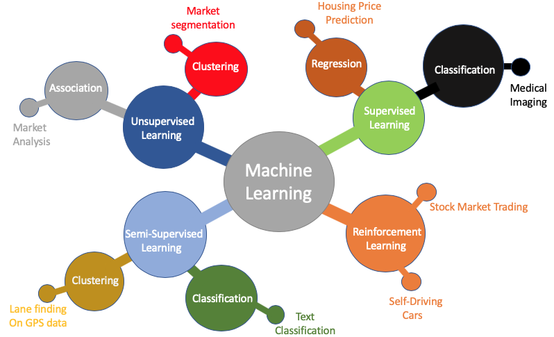
There are various types of Machine Learning. From the diagram below, you can see the main branches of Machine Learning:

Machine Learning, Robotics and Control theory is a branch of Artificial Intelligence. Machine Learning is divided into supervised, unsupervised, semi-supervised and reinforcement learning.
Supervised Learning
Supervised learning is where the algorithm is trained using the correct target values. In this algorithm, we do the training on the data and we calculate the difference between the predicted values and the correct values as the error. Regression and classification algorithms are the 2 main branches of supervised learning. Regression is where the supervised algorithm is predicting a continuous problem, such as the prediction of housing prices. Classification is where the algorithm tries to predict discrete values for example, 0 or 1, malignant or benign tumor, spam or non-spam emails.
In Machine Learning data attributes are called features. In housing prices prediction, we might use features such as house size, the number of bedrooms, the number of bathrooms, proximity to downtown, etc. Regression algorithms can perform classifications too. One of the most commonly used algorithms for classification is Logistic Regression. It gives the probabilities of belonging to a class. Some examples of supervised learning algorithms are: Linear Regression. Logistic regression Neural Networks. K- Nearest neighbors. Support Vector Machines. Decision trees and random forests.
Unsupervised Learning
Unsupervised learning is an algorithm where we make predictions using unlabeled data. In this algorithm, we use data to study the patterns to cluster data based on their similarities. Some unsupervised learning algorithms are: Clustering- K Means, Hierarchical Cluster Analysis, Expectation Maximization. Principal Component Analysis (PCA). An example of unsupervised learning use case is Google clustering related news from different sources under one URL link, market segmentation, social network analysis and astronomical data analysis. One important task in dimensionality reduction is the reduction of the number of features in our dataset while also keeping the most important features. We can ensure we keep important features by combining parameters, for example, the square feet of a house is more important than the width of the house. Some factors combined might be more important than one factor, such as age and some illnesses.
Semi-supervised learning
This is the algorithm where some data is labeled while some data is unlabeled. A great example is when we upload photos on Facebook with the same person the algorithm recognizes them. After applying a label to the person, the algorithm will name all the pictures with the same person. One example of semi-supervised learning is the deep belief networks, which is composed of unsupervised Restricted Boltzmann machines stacked on top of each other.
Reinforcement Learning
Reinforcement learning is a much deeper type of algorithm. In this algorithm, the learning system, called an agent, observes the environment, select and perform actions, and get rewards or penalties in the form of negative rewards. The best strategy, called policy defines what action the agent needs to take overtime to maximize rewards. We can use reinforcement learning in the stock market where the algorithm’s reward is to maximize the returns, and the system figures out what the best actions are to maximize the profits while it is getting negative rewards for losses.
In the programming exercises, we will use Octave software. This is the same as Matlab but it is a free open source software. This is because Octave/ Matlab makes it easy to prototype than using Java/ C++ which takes a lot of code to do. It is therefore advisable to know a prototyping language then after there is proof it works, we can move to the more complicated programming languages such as C++. After proving the code works in Octave, I will move to Python to write my algorithms. Linear Regression This is the simplest type of Supervised learning where a model is used to predict a continuous value. The well known example is the Portland housing price prediction. For the housing price prediction we use a housing price, we will use the housing price dataset.
Linear Regression
Linear regression is a supervised learning algorithm where we make predictions using a model that fits linearly on the data. Regression comes from the fact that the prediction output values are continuous. Some of the most common notations used in Machine Learning are: m - Number of training examples. x - Input variables y - Output variables (x,y)- one training example, showing the input and output. The data that is used to train the algorithm is called the training set.
| Size in Ft. squared | Price in dollars (‘000) |
|---|---|
| 1200 | 720 |
| 500 | 320 |
| 5000 | 1000 |
The main objective in Machine Learning is finding a relationship that matches the features in the first column to the output, then use this relationship to predict other outcomes given different features. Given the sizes of the houses and prices of the houses, a Supervised Learning algorithm would come up with a hypothesis that fit the features to the output in the most accurate way.
We represent the hypotheses as: \[h_\theta(x)={\theta_0} + {\theta_1 x}\]
Most of you would remember this equation is similar to y = mx + C, which is the equation of a straight line. This is the simplest algorithm to start with. Later on, we will move to algorithm equations with more than one feature as well as non-linear fuctions. In this equation, \(\theta\) are called parameters and x is the feature.
Cost function
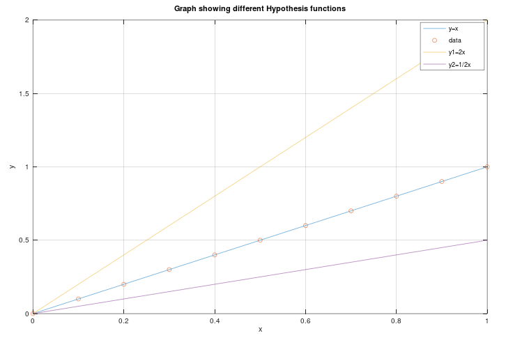
From the hypothesis function, we know that different \(\theta\) parameters, will yield different linear curves/hypothesis functions. By using different \(\theta\) parameters, we are able to fit the curves differently to different data.
The image below shows equations y = x, y = 2x and y = 1/2x. The objective is to find the best fitting plot given data as shown below:

By using different \(\theta\) parameters, we are able to come up with the line the best fits the data. This isachieved by minimizing the difference between the correct values and hypothesis predictions.
The cost function is defined as:
\[J(\theta_0, \theta_1) = \frac{1}{2m}\sum_{i=1}^{m}(h_\theta(x{^i})) - y^i)^2\]
Where m is the number of training example and i is the number of training example on the list. From the equation, the objective is to minimize the difference between the hypothesis and the correct value, y. This mathematical equation minimizes the error in the algorithm. The square in the equation is to simplify the differentiation of backpropagation. This cost function is called the square error function and it is the most commonly used cost function for regression problems.
Below are graphs showing simple cost functions and how the optimal \(\theta\) values that minimize the hypothesis functions are achieved. These graphs have only one theta values, which means one feature. A sanity check for convergence of the algorithm is plotting cost function J((\theta\)) versus \(\theta\). If the algorithm is correct, the error should be reduced with an increase in gradient descent steps. Later on, we will discuss factors such as variance and bias which assist in avoid underfitting and overfitting problems.

For graphs with more that one feature, more than one \(\theta\) parameter, it is not easy to visualize the cost function. To visualize this, a contour plot if used to check for the convergence or just a plot of cost function versus \(\theta\) and then we check if the plot is reducing with each iteration.
Gradient descent is an optimization technique that is used to find optimal solutions to a wide range of problems. It basically tweaks the parameters iteratively, until the function is minimized. This minimization algorithm is not only used in Linear Regression, but also to other algorithms such as Logistic Regression, Neural Networks to name a few.
How Gradient descent works: Start with some random values: \(\theta_0\), \(\theta_1\) Keep changing \(\theta_0\), \(\theta_1\) to reduce J(\(\theta_0\), \(\theta_1\)) until a minimum is achieved.
One issue with gradient descent is that you could end up at a local optimum. However, for linear regression, this is not a problem as they are convex functions, which means that if you pick two points and draw a line between them, the line does not cross the curve.
Gradient descent is implemented using the following equations:
\[\theta_j :=\theta_j -\alpha\frac{\partial}{\partial \theta_j} J(\theta_0,\theta_1 )\]
Then corrently simultaneously update: \[temp0 :=\theta_0-\alpha\frac{\partial}{\partial \theta_0} J(\theta_0,\theta_1 )\]
\[temp1 :=\theta_1-\alpha\frac{\partial}{\partial \theta_1} J(\theta_0,\theta_1 )\]
\[\theta_0 := temp0\] \[\theta_1 := temp1\]
:= is used to assign the new value as the current with each iteration. Care must be taken not to use the + instead as it will make them equal. \(\alpha\) is the Learning rate, which tells the algorithm how big a step to take between iterations. The \(\theta_0\) and \(\theta_1\) have to be updates simultaneously, so that new values are used during each iteration. The \(\frac{\partial}{\partial \theta_0}\) is called the partial derivative. It is similar to the normal derivative, but it is used in Calculus when we have more than one parameter such as in this example where we have \(\theta_0\) and \(\theta_1\). All that it does is to find the slope of the curve at a particular point.
A couple of points regarding the learning rate, \(\alpha\):
-
The learning rate should not be chosen to be too small as it will increase computation time, while a large learning rate will make the algorithm take big steps and might not be able to converge since it will be overshooting in each iteration and might diverge instead and never reach a global minimum. We will discuss more on this later on.
-
There is no need to decrease the learning rate with each iteration, because the slope reduces with each iteration, therefore the learning rate is automatically reduced with each iteration.
Putting it all together: Putting together the gradient descent and the cost function gives us the Linear regression algorithm. Gradien decent is used to minimize the cost function.
We should dig deeper into what the partial derivative is. What is \(\frac{\partial}{\partial \theta_j}J(\theta_0,\theta_1 \)?
\[\frac{\partial}{\partial \theta_j}J(\theta_0,\theta_1) = \frac{\partial}{\partial \theta_j} \frac{1}{2m}\sum_{i=1}^{m}(h_\theta(x{^i})) - y^i)^2\]
for \(\theta_0\) \[ j = 0 : \frac{\partial}{\partial \theta_0} J (\theta_0,\theta_1) =\frac{1}{m}\sum_{i=1}^{m}(h_\theta(x{^i})) - y^i)\]
for \(\theta_1\) \[ j = 1 : \frac{\partial}{\partial \theta_1} J (\theta_0,\theta_1) =\frac{1}{m}\sum_{i=1}^{m}(h_\theta(x{^i})) - y^i).X^i\]
The derivatives for the functions are got using Chain rule from calculus. The gradient descent that we will be using in the subsequent exercises is batch gradient decent. This means that in each step of gradient descent, both forward propagation and backpropagation are computer for all training examples. Therefore, with each iteration, all the training examples are computed using this equation \(\frac{1}{2m}\sum_{i=1}^{m}(h_\theta(x{^i})) - y^i)^2\)
Worth mentioning are other forms of gradient descent that do not run through the entire training set at once. Other types of gradient descent are stochasatic gradient descent and mini-batch gradient descent, which we will discuss later in greater detail.
Some of the references that will assist anyone who is new to Machine Learning get to speed are the following: Coursera course by Andrew Ng’- https://www.coursera.org/learn/machine-learning Tyler Rennelle blog- http://ocdevel.com/mlg
Stay tuned for the next posts for where we will go through an example of Linear Regression coding and explanations using Octave/Matlab software.
References:
1). Hands on Machine Learning with Scikit-Learn & TensorFlow by Aurelion Geron. 2). Coursera course- Machine Learning by Andrew Ng’.